Rank is a map, not a number
"What's my rank for coffee shop?" is a malformed question. Not a hard one — malformed, in the way that "how far away is it?" is malformed until you say from where. Local rank is a function of the searcher's location, and until you supply that location the question has no answer. It has a range of answers, and somebody has quietly picked one for you.
This chapter replaces the number with the right object: a field of positions across an area. Once you see rank as a surface, most of the arguments in local SEO reporting resolve themselves.
The question has a missing argument
When someone searches for a plumber, Google knows where they are. It does not ask. On a phone it is device location; on a laptop it is the network address, or a place the browser remembered, or a city the person typed.
That location is an input to ranking, not a filter applied afterwards. The three forces include distance, and distance is measured from the searcher, not from you. Change the searcher's position by a mile and you have changed one of the three inputs.
So the honest signature of a local rank is not rank(keyword). It is closer to rank(keyword, latitude, longitude, moment, language). A rank tracker that prints one number has silently frozen four of those five arguments and shown you the value at a single coordinate.
Which coordinate? Almost always the business's own address — a reasonable default, and also the single most flattering point on the map, because it is where your distance term is zero and every competitor's is not. The number on a conventional rank report is, by construction, close to your best possible result. Nobody is lying. The instrument is pointed at the one spot where the news is good.
Proximity decay
Walk away from the front door and your position degrades. This is not a penalty and it is not something you did wrong — it is arithmetic. Every step away from your own address moves some competitor closer to the searcher than you are, and Google re-sorts accordingly.
The previous chapter put published magnitudes on that decay, along with the reasons those magnitudes are softer than they look. The point here is structural rather than numeric: whatever the decay curve is, one number cannot represent a surface.
Two things make that surface less tidy than the word "decay" suggests.
It is not a circle. Decay follows competitor density, not geometry. If every rival clusters on one side of town, your visibility extends much further in the other direction. A river, a motorway or a city boundary can produce a sharp edge. (Inference — a pattern practitioners read routinely in grids, not something Google documents.)
It is not smooth. Rank is a sort order, and a sort order jumps. Two points 400 metres apart can differ by six positions because that step reordered three businesses whose scores were nearly tied.
A geo-grid is the instrument
Sample the field, do not take one reading. A geo-grid measures rank the way you would measure temperature across a room: sample it at many points and look at the field.
The procedure is four steps:
- Pick a centre.
- Lay out an n×n lattice of points at a fixed spacing.
- Run the same search from each point, as though a person were standing there.
- Record where the business appears.
What you get back is n² positions with coordinates attached. Drawn on a map with colour, that is a heatmap.
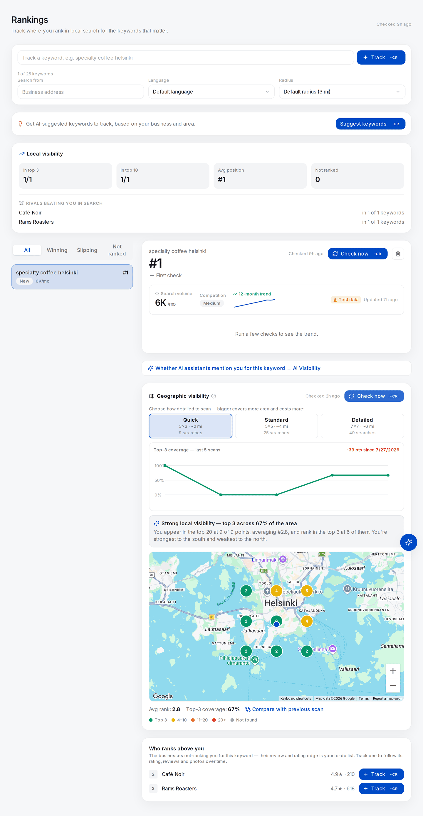
A real scan, not an illustration: nine live searches for one keyword, one from each point, run within a minute of each other. The pins carry different positions depending only on where the searcher is standing — that spread is the entire subject of this chapter.
The two figures under the map compress all nine into Avg rank 2.8 and Top-3 coverage 67%. Look at the small trend strip above the map before you trust either of them: it plots five scans of these same nine points taken across a single day, and it reads 100%, 0%, 0%, 67%, 67%. Nothing about the business changed between them. Part III is about what to do with an instrument that behaves like that.
Doing it by hand is possible and instructive — an incognito window plus a location override in your browser's dev tools produces one grid point at a time, and twenty-five of them is an afternoon. See Doing all of this without SEOG.
Two knobs, not one
A grid has two independent parameters doing different jobs.
- Extent — how much ground the grid covers. It tells you where your visibility ends.
- Spacing (resolution) — how far apart the points are. It tells you how fine a feature the grid can see.
Independent in principle; not in the app, where grid points are spaced one mile apart and the preset sets n. So the three presets change extent, and only extent.
| Preset | Grid | Points | Span at one-mile spacing |
|---|---|---|---|
| Quick | 3×3 | 9 | ~2 mi across |
| Standard | 5×5 | 25 | ~4 mi across |
| Detailed | 7×7 | 49 | ~6 mi across |
This is a real limitation and worth naming: a one-mile grid cannot answer a question about half a mile. If you want to know which side of the high street you win, no preset here will tell you — you need tighter spacing, which means running the points yourself. A grid resolves nothing smaller than its own step size.
An n×n scan is exactly n² live searches. Nine for 3×3, twenty-five for 5×5, forty-nine for 7×7. Not "about" — each point is one independent search run from that point's coordinates.